Problem Set 8
Due at 3:00 pm on Tuesday, Apr. 30. Please submit to Gradescope and follow the general guidelines regarding homework assignments.
Unfolding in time
Define a recurrent net by \(\begin{align} \vec{h}_{t} &= f (W \vec{h}_{t - 1} + U \vec{x}_t)\\ \vec{y}_{t} &= g (V\vec{h}_t) \end{align}\) for \(t=1\) to \(T\) with initial condition \(\vec{h}_{0} =0\). At time \(t\),
- \(\vec{x}_t\) is the \(d_x\)-dimensional activity vector for the input neurons (input vector),
- \(\vec{h}_t\) is the \(d_h\)-dimensional activity vector for the hidden neurons (hidden state vector),
- and \(\vec{y}_t\) is the \(d_y\)-dimensional activity vector for the output neurons (output vector).
The network contains three connection matrices:
- The \(d_h\times d_x\) matrix \(U\) specifies how the hidden neurons are influenced by the input,
- the \(d_h\times d_h\) “transition matrix” \(W\) governs the dynamics of the hidden neurons,
- and the \(d_y\times d_h\) matrix \(V\) specifies how the output is “read out” from the hidden neurons.
The network can be depicted as
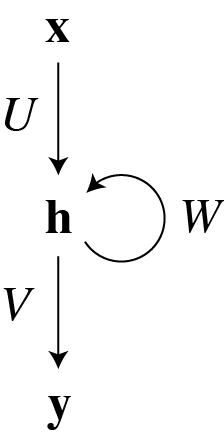
where the recurrent connectivity is represented by the loop. Note that if \(W\) were zero, this would reduce to a multilayer perceptron with a single hidden layer.
If we want to run the recurrent net for a fixed number of time steps, we can unfold or unroll the loop in the above diagram to yield a feedforward net with the architecture:
\[\require{AMScd} \begin{CD} @. \vec{x}_1 @. \vec{x}_2 @. \cdots @. \vec{x}_T\\ @. @VU_1VV @VU_2VV @VVV @VU_TVV\\ \vec{h}_0 @>W_1>> \vec{h}_1 @>W_2>> \vec{h}_2 @>>> \cdots @>W_T>> \vec{h}_T\\ @. @V{V_1}VV @V{V_2}VV @VVV @V{V_T}VV\\ @. \vec{y}_1 @. \vec{y}_2 @. \cdots @. \vec{y}_T\\ \end{CD}\]In this diagram, we temporarily imagine that the connection matrices \(W_t\), \(U_t\), and \(V_t\) vary with time: \(\begin{align} \vec{h}_{t} &= f (W_t \vec{h}_{t - 1} + U_t \vec{x}_t)\\ \vec{y}_{t} &= g (V_t\vec{h}_t) \end{align}\) This reduces to the recurrent net in the case that \(W_t=W\) for all \(t\) (and similarly for the other connection matrices). This is called “weight sharing through time.”
The diagram has the virtue of making explicit the pathways that produce temporal dependencies. The last output \(\vec{y}_T\) depends on the last input \(\vec{x}_T\) through the short pathway that goes through \(\vec{h}_T\). The last output also depends on the first input \(\vec{x}_1\) through the long pathway from \(\vec{h}_1\) to \(\vec{h}_T\).
Backpropagation through time
The backward pass can be depicted as
\[\require{AMScd} \begin{CD} @. \tilde{\vec{x}}_1 @. \tilde{\vec{x}}_2 @. \cdots @. \tilde{\vec{x}}_T\\ @. @A{U_1^\top}AA @A{U_2^\top}AA @AAA @A{U_T^\top}AA\\ \tilde{\vec{h}}_0 @<{W_1^\top}<< \tilde{\vec{h}}_1 @<{W_2^\top}<< \tilde{\vec{h}}_2 @<<< \cdots @<{W_T^\top}<< \tilde{\vec{h}}_T\\ @. @A{V_1^\top}AA @A{V_2^\top}AA @AAA @A{V_T^\top}AA\\ @. \tilde{\vec{y}}_1 @. \tilde{\vec{y}}_2 @. \cdots @. \tilde{\vec{y}}_T\\ \end{CD}\]Here \(\tilde{\vec{h}}_t\) is the backward pass variable that corresponds with the forward pass preactivity \(f^{-1}(\vec{h}_t)\) (and similarly for other tilde variables).
Exercises
-
Write the equations of the backward pass corresponding to the diagram. As a concrete example, use the loss \[ E = \sum_{t=1}^T \frac{1}{2}|\vec{d}_t - \vec{y}_t|^2 \] where \(\vec{d}_t\) is a vector of desired values for the output neurons at time \(t\). The equations for \(\tilde{\vec{x}}_t\) and \(\tilde{\vec{h}}_0\) won’t be used in the gradient descent updates, but write them anyway. (They would be useful if \(\vec{x}^t\) were the output of other neural net layers and we wanted to continue backpropagating through those layers too.)
-
In the gradient descent updates, \(\begin{align} \Delta U_t &\propto \tilde{\vec{h}}_?\vec{x}_?^\top\\ \Delta W_t &\propto \tilde{\vec{h}}_?\vec{h}_?^\top\\ \Delta V_t &\propto \tilde{\vec{y}}_?\vec{h}_?^\top \end{align}\) supply the missing letters where there are question marks. Note how the backward pass diagram above shows the paths by which the loss at time \(t\) can influence the gradient updates for previous times.
-
To obtain the backprop update for the recurrent net, we must enforce the constraint of weight sharing in time (\(W_t=W\) for all \(t\), etc.). Write the gradient updates for \(U\), \(V\), and \(W\).
Backprop with multiplicative interactions
Consider the feedforward net, \(\begin{align} \vec{x}^1 &= f(W^{1x}\vec{x}^0 + \vec{b}^{1x})\\ \vec{y}^1 &= f(W^{1y}\vec{y}^0 + \vec{b}^{1y})\\ \vec{z}^1 &= \vec{x}^1.*\vec{y}^1\\ \vec{z}^2 &= f(W^2\vec{z}^1 + \vec{b}^2) \end{align}\)
The vectors represent the layer activities, and superscripts indicate layer indices. The elementwise multiplication of \(\vec{x}^1\) and \(\vec{y}^1\) makes this net different from a multilayer perceptron.
Exercises
- Write the backward pass for the net.
- Write the gradient updates for the weights and biases.
Programming exercises
- Here you will use a recurrent net to predict the next character in the Shakespeare corpus. It won’t produce samples indistinguishable from Shakespeare, but some structure should emerge from training.
-
Experiment with sampling from the model with different temperature parameters. Show one sample with temperature very close to 0 and one with an extremely high temperature. What does temperature qualitatively do to the samples? Report a temperature that produces comparatively nice results and show its output.
-
Repeat the experiment switching to
nn.LSTM. How the training is different? Report the final cross entropy per letter on the training set. -
If you want to reduce the cross entropy per letter and/or generate better samples you could train for longer and experiment with the optimization parameters by altering learning rate through the training. Make some alterations to the training procedure that you think will improve performance and describe why.
-
Train using your modified procedure. Once training is done, calculate the cross entropy per letter on the training set. Is this better or worse than the Elman/LSTM net?
-
- Cell types
We already used Pytorch ready implementation of Elman (simple RNN) and LSTM cells, now we will implement them ourselves.
- Implement Elman network.
- Implement LSTM network.
- Describe the role of each gate in the LSTM network.
- What is the difference between Elman and LSTM networks? Which one is better at generating Shakespeare, and why?
- (EXTRA) Modify CharRNN object to take your implemented module and run it using the training procedure from above. Show some output. Be careful with modifications.